Table of Contents
The degrees of freedom (DF) formula indicates the number of independent values that can vary in an analysis without breaking any constraints. It is an important concept that appears in many contexts in statistics, including hypothesis tests, probability distributions, and linear regression. Find out how this concept affects your analysis’ power and precision!
In this post, I explain this concept in an intuitive way. During this class, you will learn the definition of degrees of freedom and how to calculate degrees of freedom for various analyses, such as linear regression, t-tests, and chi-square. My first step will be to define degrees of freedom and provide a formula. As an alternative, I will present practical examples in the context of various statistical analyses because they provide a better understanding of the concept.
Degrees Of Freedom
In statistics, degrees of freedom are important concepts in hypothesis testing, regression analysis, and probability distributions.
By subtracting one from the total number of observations in a statistical sample, one can estimate parameters. Applications of the calculation can be found in businesses, economics, and finance.
Degrees Of Freedom Formula Calculator
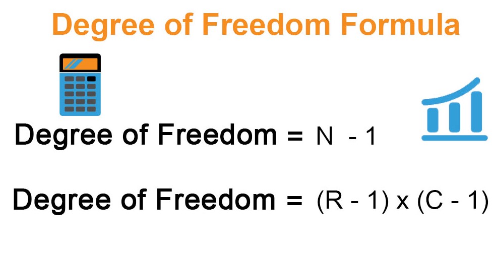
The formula to calculate degrees of freedom is:
df = N – 1
Where:
- df = degrees of freedom
- N = sample size
To calculate the degrees of freedom for a given sample size, simply subtract 1 from the sample size.
For example, if you have a sample size of 20, the degrees of freedom would be:
df = 20 – 1 df = 19
Therefore, the degrees of freedom for a sample size of 20 is 19.
You can use this formula to calculate degrees of freedom for any sample size.
Degrees Of Freedom Statistics Formula
In statistics, the formula for degrees of freedom depends on the type of test or analysis being performed. Here are some common formulas for calculating degrees of freedom in various statistical tests:
- T-test: The formula for degrees of freedom in a two-sample t-test is:
df = n1 + n2 – 2
Where:
- df = degrees of freedom
- n1 and n2 = sample sizes of the two groups being compared
- Chi-square test: The formula for degrees of freedom in a chi-square test is:
df = (r – 1) x (c – 1)
Where:
- df = degrees of freedom
- r = number of rows in the contingency table
- c = number of columns in the contingency table
- ANOVA: The formula for degrees of freedom in a one-way ANOVA is:
df = k – 1
Where:
- df = degrees of freedom
- k = number of groups being compared
The formula for degrees of freedom in a two-way ANOVA is:
df = (n – 1) – (a + b – 2)
Where:
- df = degrees of freedom
- n = total sample size
- a = number of levels in the first factor
- b = number of levels in the second factor
These are just a few examples of formulas for calculating degrees of freedom in statistics. It’s important to use the correct formula for the specific test or analysis you are conducting in order to obtain accurate results.
Degrees Of Freedom Formula Chi Square
The formula to calculate degrees of freedom for a chi-square test is:
df = (r – 1) x (c – 1)
Where:
- df = degrees of freedom
- r = number of rows in the contingency table
- c = number of columns in the contingency table
The chi-square test is used to determine whether there is a significant association between two categorical variables. The contingency table is used to organize the data into rows and columns based on the categories being analyzed. The degrees of freedom in this test represent the number of independent pieces of information that can be used to estimate the expected frequencies in the contingency table.
For example, if you have a contingency table with 3 rows and 4 columns, the degrees of freedom would be:
df = (3 – 1) x (4 – 1) df = 2 x 3 df = 6
Therefore, the degrees of freedom for a chi-square test with a contingency table of 3 rows and 4 columns is 6.
The Formula For The Degrees Of Freedom For The Dependent-samples T Test Is:
The formula for the degrees of freedom for the dependent-samples t-test is:
df = n – 1
Where:
- df = degrees of freedom
- n = number of pairs of scores
The dependent-samples t-test is used to compare the means of two related groups, such as before and after measurements of the same individuals or matched pairs. The degrees of freedom in this test represent the number of independent pieces of information available to estimate the population standard deviation.
For example, if you have a sample of 10 pairs of scores, the degrees of freedom would be:
df = 10 – 1 df = 9
Therefore, the degrees of freedom for a dependent-samples t-test with 10 pairs of scores is 9.
What Is the Degree Of Freedom?
\(\mathbf{\color{red}{Degrees\ of\ freedom\ (df)\ refers\ to\ the\ number\ of\ independent\ values\ (variable)\\ in\ a\ data\ sample\ used\ to\ find\ the\ missing\ piece\ of\ information\ (fixed)\ without\\ violating\ any\ constraints\ imposed\ in\ a\ dynamic\ system.\ These\ nominal\ values\\ have\ the\ freedom\ to\ vary,\ making\ it\ easier\ for\ users\ to\ find\ the\ unknown\\ or\ missing\ value\ in\ a\ dataset.}}\)
The degrees of freedom in a statistical calculation represents the number of values that can be varied in a calculation. To ensure the statistical validity of chi-square tests, t-tests, and even the more advanced f-tests, degrees of freedom can be calculated. Data from these tests are commonly used to compare observed data with data that would be expected to be obtained according to a specific hypothesis.
Let’s say that a drug trial is conducted on a group of patients, and it is hypothesized that the patients receiving the drug will have higher heart rates than those who do not receive it. The results of the test could be analyzed to determine whether the difference in heart rates is considered significant, and degrees of freedom are included in the calculation.
Degrees of freedom calculations identify how many values in the final calculation can vary, so they contribute to the validity of an outcome. The calculations depend on the number of observations and the parameters to be estimated, but generally, in statistics, degrees of freedom equal the number of observations minus the number of parameters. As sample sizes increase, more degrees of freedom become available.
How to Find the Degrees of Freedom in Statistics
That last number has no room for variation, as you can see. It is not an independent piece of information because it cannot be of any other value. In an attempt to estimate the parameter, the mean, in this case, constrains the freedom of variation last value since the mean is entirely interdependent. consequently, even with a sample size of 10, we only have 9 independent pieces of information after estimating the mean.
DF in statistics is based on that basic idea. In a general sense, DF is the number of observations that are free to vary when estimating statistical parameters. It can also be thought of as the amount of independent data you can use to estimate a parameter.
Degrees Of Freedom Formula Thermodynamics
In thermodynamics, the degrees of freedom refer to the number of independent ways that a molecule or system can store energy or move. The degrees of freedom formula for a monoatomic gas is given by:
f = 3
where “f” is the number of degrees of freedom. This means that a monoatomic gas molecule can store energy in three ways: translational motion along the three orthogonal axes.
For a diatomic gas, the degrees of freedom formula is given by:
f = 5
where the two additional degrees of freedom arise from the ability of the molecule to rotate about two axes perpendicular to its axis of symmetry. In addition to the three translational degrees of freedom, the diatomic gas molecule has two additional rotational degrees of freedom.
For a polyatomic gas, the degrees of freedom formula can be calculated using the following equation:
f = 3N – 6
where “N” is the number of atoms in the molecule. This equation takes into account the three translational degrees of freedom for each atom, minus the six degrees of freedom associated with the overall translation and rotation of the molecule as a whole. The remaining degrees of freedom are associated with the internal vibrational and rotational modes of the molecule.
Degrees Of Freedom Formula Chemistry
In chemistry, degrees of freedom typically refer to the number of ways that a molecule can move or vibrate. The number of degrees of freedom is determined by the number of atoms in the molecule and the type of motion that is considered.
For example, a molecule with “n” atoms has 3n degrees of freedom associated with its motion in three-dimensional space. These degrees of freedom include translational, rotational, and vibrational motion.
The formula for the degrees of freedom in chemistry can be given as:
f = 3n – r
where “f” is the number of degrees of freedom, “n” is the number of atoms in the molecule, and “r” is the number of constraints on the motion of the molecule. Constraints can arise due to the presence of chemical bonds, molecular symmetry, and other factors.
For example, a diatomic molecule such as H2 has two atoms, so the number of degrees of freedom is:
f = 3(2) – 2 = 4
This means that the molecule can move in four ways: it can translate along the x, y, and z axes, and it can rotate about its center of mass.
In more complex molecules, the number of degrees of freedom can be much larger. The formula for degrees of freedom in chemistry can be used to determine the number of vibrational modes and rotational modes that are available to the molecule, which can have important implications for its properties and reactivity.
Degrees Of Freedom Formula For Gases
The degrees of freedom formula for gases is derived from the ideal gas law, which describes the relationship between the pressure, volume, and temperature of a gas. According to the kinetic theory of gases, the molecules of a gas are in constant motion and have translational, rotational, and vibrational degrees of freedom.
The formula for the degrees of freedom for a gas molecule can be given as:
f = 3N – c
where “f” is the number of degrees of freedom, “N” is the number of atoms or molecules in the gas, and “c” is the number of constraints on the motion of the gas.
For an ideal gas consisting of monatomic molecules (such as helium or neon), the gas particles have only translational degrees of freedom. Therefore, the number of degrees of freedom is simply equal to three times the number of gas molecules:
f = 3N
For a gas consisting of diatomic molecules (such as oxygen or nitrogen), the gas particles have additional rotational degrees of freedom. In this case, the number of degrees of freedom is:
f = 3N – 3
This is because each diatomic molecule has three rotational modes (two around the axis perpendicular to the bond and one around the bond axis), which reduces the number of translational degrees of freedom by three.
For more complex gas molecules, such as those with multiple atoms or non-linear shapes, the number of degrees of freedom can be more complicated to calculate. However, the basic principle remains the same: the number of degrees of freedom is equal to three times the number of atoms or molecules minus the number of constraints on their motion.
The Formula For Degrees Of Freedom
Degrees of freedom are easy to calculate. Degrees of freedom are often calculated by subtracting the sample size from the number of parameters you are estimating:
$$DF = N – P$$
Where:
\(N\) = sample size
\(P\) = the number of parameters or relationships
The degrees of freedom formula for a 1-sample t-test is \(N – 1\) since you’re estimating one parameter, the mean. Use \(N – 2\) to calculate degrees of freedom in a two-sample t-test, since there are now two parameters to estimate.
The degrees of freedom formula for a table in a chi-square test is \((r-1) (c-1)\), where \(r\) is the number of rows and \(c\) is the number of columns.
DF and Probability Distributions
Degrees of freedom also determine the probability distributions for the test statistics of various hypothesis tests. To determine statistical significance, hypothesis tests use the t-distribution, F-distribution, and chi-square distribution. Each of these probability distributions is a family of distributions in which the DF determines the shape. These distributions are used to calculate p-values for hypothesis tests. Thus, the DF is directly linked to p-values through these distributions!
Let’s look at how these distributions work for several hypothesis tests.
Degrees of Freedom Table
In statistical tables, you’ll often see degrees of freedom along with their critical values. The DF in these tables is used by statisticians to determine whether the test statistic for their hypothesis test falls within the critical region, indicating statistical significance.
You can find the degrees of freedom in the first column of a t-table, for example. It is necessary to know these degrees of freedom in order to calculate the critical values. The t-table below shows that for a two-tailed t-test with \(20 DF\) and an alpha of \(0.05\), the critical values are \(-2.086\ and\ +2.086\).
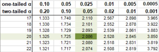
The critical t-value for a two-sided t-test according to the T-distribution table.
For other hypothesis tests, such as the chi-square, F-tests, and z-tests, there are tables where you can find the degrees of freedom and the corresponding critical values.
- Z-table
- F-table
- Chi-square table
Critical Values
The degrees of freedom for a population or for a sample doesn’t provide much useful information by themselves. Using a critical value table, we can find the critical values for our equation after we calculate the degrees of freedom, which is the number of values in a calculation that can be varied. These tables can be found in textbooks and online. Using a critical value table, the values in the table determine the statistical significance of the results.
Chi-square tests and t-tests are examples of how degrees of freedom can be used in statistical calculations. Different t-tests and chi-square tests can be differentiated by using degrees of freedom.
Why Do Critical Values Decrease While DF Increase?
Take a look at the t-score formula in a hypothesis test:
$$\mathbf{\color{red}{t=\frac{\bar{x}-{\mu_0}}{\frac{s}{\sqrt n}}}}$$
When n increases, the t-score goes up. This is due to the square root in the denominator: as it gets larger, the fraction \(\frac{s}{\sqrt n}\) gets smaller and the t-score (the result of another fraction) gets bigger. Considering the degrees of freedom above as n-1, you would expect the t-critical value to get bigger as well, but they don’t: they get smaller. It seems counterintuitive.
However, consider what a t-test is really for. The t-test is used because you don’t know the standard deviation of your population and therefore don’t know the shape of your graph. It could have short tails. The tails could be long and skinny. The possibilities are endless.
Degrees of freedom affect the shape of the graph in the t-distribution; as df increases, the tails of the distribution become smaller. The t-distribution will resemble a normal distribution as df approaches infinity. You can determine your standard deviation (which is 1 on a normal distribution) when this happens.
T-Test Formula
There are three types of t-tests described in this article: one-sample, two independent samples, and paired samples tests. The formula for the t-test is also known as:
- T-test Equation,
- T-score Equation,
- T-test Statistic Formula
- Formula For T-test
One Sample T-test Formula
A one-sample t-test is used to compare the mean of one sample with a known standard mean. This is how one-sample t-tests are expressed:
$$\mathbf{\color{red}{t = \frac{m-\mu}{\frac{s}{\sqrt{n}}}}}$$
where,
\(\mathbf{\color{red}{m}}\) is the sample mean
\(\mathbf{\color{red}{n}}\) is the sample size
\(\mathbf{\color{red}{s}}\) is the sample standard deviation with \(\mathbf{n−1}\) degrees of freedom
\(\mathbf{\color{red}{\mu}}\) is the theoretical mean
The p-value, which corresponds to the absolute value of the t-test statistic \((|t|)\), is calculated using the degrees of freedom \((df)\): $$\mathbf{\color{red}{df = n – 1}}$$
How to interpret the one-sample t-test results?
We can reject the null hypothesis and accept the alternative hypothesis if the p-value is less than or equal to the significance level of \(0.05\). Therefore, the sample mean is significantly different from the theoretical mean.
Independent T-test Formula
Two independent groups are compared using the independent t-test formula. There are two types of independent t-tests:
- The Student’s t-test assumes that the variances of the two groups are equal.
- In contrast to the original Student’s test, the Welch’s t-test is less restrictive. In this test, you do not assume that the variance in the two groups is the same, resulting in fractional degrees of freedom.
This article explains the Student t-test formula and the Weltch t-test formula.
Student T-test Formula
Assuming that the variances of the two groups are equivalent (homoscedasticity), the t-test value, comparing the two samples \((A\ and\ B)\), can be calculated as follows.
$$\mathbf{\color{red}{t = \frac{m_A – m_B}{\sqrt{ \frac{S^2}{n_A} + \frac{S^2}{n_B}}}}}$$
where,
\(\mathbf{\color{red}{m_A\ and\ m_B}}\) represent the mean value of groups \(A\) and \(B\), respectively.
\(\mathbf{\color{red}{n_A\ and\ n_B}}\) represent the sizes of groups \(A\) and \(B\), respectively.
\(\mathbf{\color{red}{S^2}}\) is an estimator of the pooled variance of the two groups. It can be calculated as follow :
$$\mathbf{\color{red}{S^2 = \frac{\sum{(x-m_A)^2}+\sum{(x-m_B)^2}}{n_A+n_B-2}}}$$
with degrees of freedom \((df)\): $$\mathbf{\color{red}{df = n_A + n_B – 2}}$$
Welch’s T Test Formula
The Welch t-test, which is an adaptation of the Student t-test, can be used if the variances of the two groups being compared differ (heteroscedasticity). Welch’s t-statistic is calculated as follows:
$$\mathbf{\color{red}{t = \frac{m_A – m_B}{\sqrt{ \frac{{S_A}^2}{n_A} + \frac{{S_B}^2}{n_B}}}}}$$
where, \(S_A and S_B\) are the standard deviations of the two groups \(A\) and \(B\), respectively.
Unlike the classic Student’s t-test, the Welch t-test formula involves the variance of each of the two groups \({S_A}^2\) and \({S_B}^2\) being compared. In other words, it does not use the pooled variance \(S\).
The degrees of freedom of Welch t-test is estimated as follow :
$$\mathbf{\color{red}{df = \frac{(\frac{S_A^2}{n_A}+ \frac{S_B^2}{n_B})^2}{(\frac{S_A^4}{n_A^2(n_A-1)} + \frac{S_B^4}{n_B^2(n_B-1)})}}}$$
A p-value can be computed for the corresponding absolute value of the t-statistic \((|t|)\).
We can reject the null hypothesis and accept the alternative hypothesis if the p-value is less than or equal to the significance level of \(0.05\). To put it another way, we can conclude that groups A and B have significantly different mean values.
It is worth noting that the Welch t-test is considered to be safer. Generally, the results of the classical student’s t-test and the Welch t-test are very similar unless the group sizes and standard deviations are quite different.
Paired T-test Formula
To compare the means of two related groups of samples, the paired t-test is used.
The procedure of the paired t-test analysis is as follows:
- Calculate the difference (d) between each pair of value
- Compute the mean (m) and the standard deviation (s) of d
- Compare the average difference to 0. If there is any significant difference between the two pairs of samples, then the mean of d (m) is expected to be far from 0.
The paired t-test statistics value can be calculated using the following formula:
$$\mathbf{\color{red}{dt = \frac{m}{\frac{s}{\sqrt{n}}}}}$$
where,
\(\mathbf{\color{red}{m}}\) is the mean differences
\(\mathbf{\color{red}{n}}\) is the sample size (i.e., size of d)
\(\mathbf{\color{red}{s}}\) is the standard deviation of d
We can compute the p-value corresponding to the absolute value of the t-test statistics \((|t|)\) for the degrees of freedom (df): $$\mathbf{\color{red}{df=n−1}}$$
If the p-value is inferior to or equal to 0.05, we can conclude that the differences between the two paired samples are significantly different.
Chi-Square Test of Independence
A Chi-Square test of independence is used to determine if there is a significant relationship between two nominal (categorical) variables. The frequency of categories for one nominal variable is compared with the frequency of categories for the second nominal variable. It is possible to display the data as a contingency table where each row represents a category for one variable and each column represents a category for the other variable.
Say a researcher wants to look at the relationship between gender (male vs. female) and empathy (high vs. low). Chi-square tests of independence can be used to investigate this relationship. According to this test, there is no relationship between gender and empathy. An alternative hypothesis is that there is a relationship between gender and empathy (i.e., more high-empathy females than high-empathy males).
How to Find Degrees of Freedom for Tables in Chi-Square Tests
A chi-square test of independence determines whether categorical variables in a table have a statistically significant relationship. This test includes \(DF\), as do other hypothesis tests. To calculate degrees of freedom for a table with r rows and c columns, use this formula: \((r-1) (c-1)\).
We can create tables to understand how to find degrees of freedom more intuitively, however. The DF of a chi-square test of independence is the number of cells in the table that have to vary before the rest of the cells can be calculated. In a chi-square table, the cells show the observed frequency of each combination of categorical variables. Constraints are the totals in the margins.
Chi-Square \(2 \times 2\) Table
When you enter one value in a \(2 \times 2\), you can calculate all the remaining cells if you want to find the degrees of freedom.
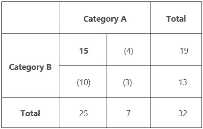
Using the table above, I entered the bolded 15 and then calculated the remaining three values in parentheses. As a result, this table has one DF.
Chi-Square \(3 \times 2\) Table
Now let’s try to find degrees of freedom for the \(3 \times 2\) table. In my post about the chi-square test of independence, I used the table below to illustrate my example. I examine whether there is a statistically significant relationship between uniform color and deaths in the original Star Trek TV series.
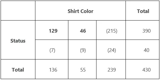
One of the categorical variables in the table is shirt color, which can be blue, gold, or red. The other categorical variable is status, which can be either dead or alive. By entering the two bolded values, I can calculate all the remaining cells. Hence, this table contains 2 DFs.
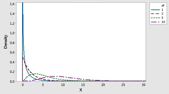
Similar to the t-distribution, the chi-square distribution is a family of distributions whose shape is defined by the DF. Chi-square tests utilize this distribution to calculate p-values. Following is a chart of several chi-square distributions.
An illustration of the distribution of chi-squared values based on different degrees of freedom.
Linear Regression Degrees of Freedom
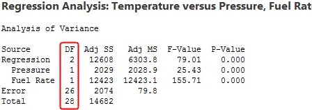
In linear regression, calculating degrees of freedom is a bit more complicated, so I will keep it simple. Each term in a linear regression model represents an estimated parameter with one degree of freedom. You can see from the regression output below that each linear regression term requires a DF. There are 29 observations, and two DF are used for both independent variables.
Degrees of freedom formula for total \(DF = n – 1\), which is \(29 – 1 = 28\) in our example. To calculate Error DF, \(n – P – 1\) is the degrees of freedom formula. In our example that is \(29 – 2 – 1 = 26\). \(P\) is the number of coefficients excluding the constant. Error displays the remaining 26 degrees of freedom.
The error DF is the independent information that can be used to estimate your coefficients in linear regression. If you want precise coefficient estimates and powerful hypothesis tests in regression, you must have many error degrees of freedom, which equates to many observations for each model term.
The error degrees of freedom decrease as you add terms to the model. As a result, you have less information available to estimate the coefficients. The precision of the estimates and the power of the tests is reduced as a result. If you have too few remaining DF, you cannot trust the regression results. The procedure cannot calculate p-values if you use all your linear regression degrees of freedom.
You can learn more about the problems that occur when you use too many DF and how many observations you need by reading my blog post about overfitting your model.
Although the definition of degrees of freedom might seem murky, they are essential to any statistical analysis! DF refers to the amount of information you have relative to the number of properties you want to estimate. If you don’t have enough data, you’ll have imprecise estimates and low statistical power.
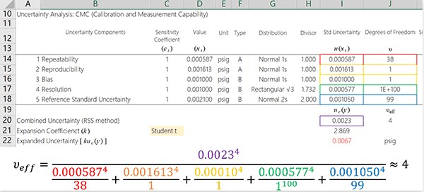
Example: Calculating Effective Degrees of Freedom
Calculating the degrees of freedom associated with uncertainty estimation is important when performing uncertainty analysis. To determine the total degrees of freedom, you cannot simply add together all of your independently calculated degrees of freedom. To determine the effective degrees of freedom, you must use the Welch-Satterthwaite approximation equation. Learn how to apply the Welch Satterthwaite approximation equation to your uncertainty analysis in this article.
If you prefer, you can check out the next section to learn how to calculate the effective degrees of freedom using Microsoft Excel.
In order to make the process of calculating effective degrees of freedom with the Welch Satterthwaite equation easier to follow, I am going to break the process down into easy steps.
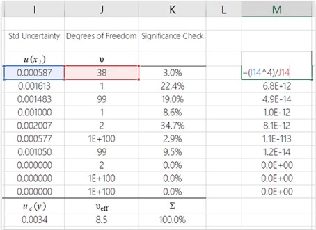
Each uncertainty component is raised to the power of \(4^1\)
First, we want to raise the standard uncertainty component to the power of 4. Here is the formula in Microsoft Excel. Copy and paste the function for the remaining uncertainty components after you have raised the first uncertainty component to the power of 4.
Power of 4 means that you multiply the uncertainty component value by itself four times or use an exponent of 4.
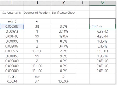
Divide each degree of freedom by its associated uncertainty
Taking your previous result and dividing it by its associated degrees of freedom is the next step.
See the image below to learn how to do this in MS Excel.
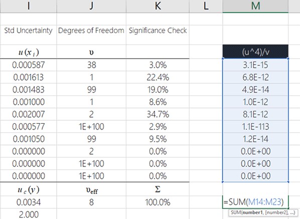
Added the results from the previous step,
In this step, you will add up all the results from the previous step.
You can easily do this in MS Excel by using the summation (SUM) function. Here is an image showing how to do it.
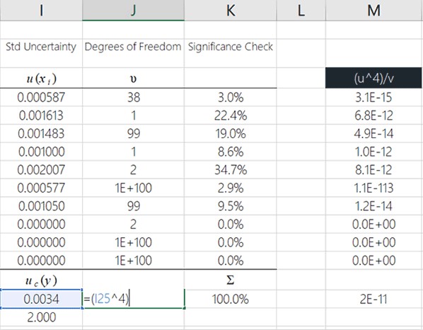
Raise the combined uncertainty to the power of 4
Now, you need to raise your combined standard uncertainty to the power of 4.
You can see how to do this in Microsoft Excel by looking at the image below. It is recommended that you enter this function where you want to see the calculated degrees of freedom because I will show you how to complete this process in the cell you see in the image below.
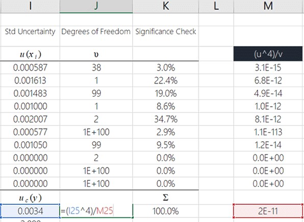
Divide the result in step 4 by the result in step 3
You will now divide the result from the previous step by the result you calculated in step 3.
To see how to do it in Microsoft Excel, look at the image below.
The degrees of freedom that you calculate is the effective degrees of freedom. This is not the end of your calculation. The result needs to be rounded to a whole number in the next step.
Round the result to the nearest whole number.
Finally, round the result to a whole number using the ROUND function in Microsoft Excel.
Look at the image below to see how to do it.

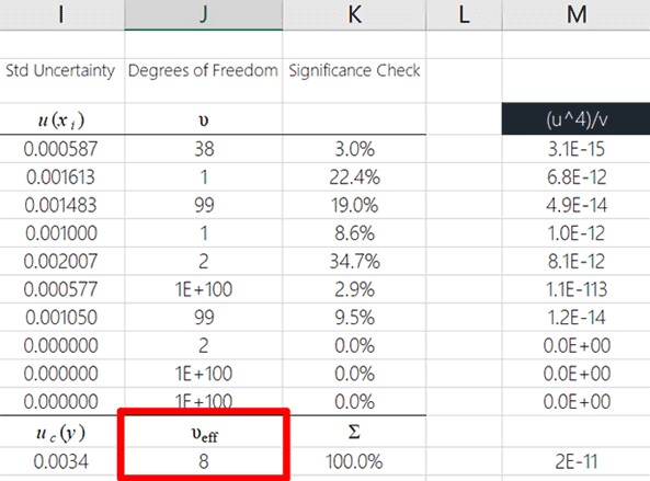
The Result
Following the steps above, you have calculated the effective degrees of freedom. Well done!
The final result can be seen in the image below.
FAQs
What is DF in at test?
Degrees of freedom (DF) is the amount of information that your data provider allows you to “spend” to estimate the values of unknown population parameters and calculate their variability. This value is determined by the number of observations in your sample.
What is the use of the degree of freedom?
A degree of freedom definition is a mathematical equation used primarily in statistics, but also in physics, mechanics, and chemistry. The number of degrees of freedom in a statistical calculation refers to the number of possible values that are involved in a calculation.
What is the role of the degree of freedom?
A degree of freedom is an integral component of inferential statistics, which estimates or makes inferences about population parameters based on sample data. Defining degrees of freedom as the number of variables that are free to vary in a calculation.
Why is the degree of freedom called?
The number of degrees of freedom in statistics refers to the number of possible values in the final calculation of a statistic. The number of independent ways by which a dynamic system can move without violating any constraints imposed on it is called its degrees of freedom.
What is K in degrees of freedom?
Degrees of freedom can be calculated as follows: \(df_1 = k-1\) and \(df_2 = N-k\), where \(k\) is the number of comparison groups and \(N\) is the total number of observations.
Which Of The Following Is The Formula Used To Calculate Degrees Of Freedom For A T Test?
The formula used to calculate degrees of freedom for a t-test depends on whether it is a one-sample t-test, independent-samples t-test, or dependent-samples t-test. Here are the formulas for each:
- One-sample t-test: df = n – 1, where n is the sample size.
- Independent-samples t-test: df = (n1 + n2) – 2, where n1 and n2 are the sample sizes of the two groups being compared.
- Dependent-samples t-test: df = n – 1, where n is the number of pairs of scores.
Therefore, the formula used to calculate degrees of freedom for a t-test depends on the specific type of t-test being conducted.
What Is The Formula Used To Calculate Degrees Of Freedom For A T-test For Dependent Groups?
The formula used to calculate degrees of freedom for a t-test for dependent groups is:
df = n – 1
Where:
- df = degrees of freedom
- n = number of pairs of scores
The t-test for dependent groups, also known as a paired t-test or repeated measures t-test, is used to compare the means of two related groups, such as before and after measurements of the same individuals or matched pairs. The degrees of freedom in this test represent the number of independent pieces of information available to estimate the population standard deviation.
For example, if you have a sample of 10 pairs of scores, the degrees of freedom would be:
df = 10 – 1 df = 9
Therefore, the degrees of freedom for a t-test for dependent groups with 10 pairs of scores is 9.
What Is The Correct Formula For Between-groups Degrees Of Freedom?
The formula for between-groups degrees of freedom, also known as the between-group variability, is:
df_between = k – 1
Where:
- df_between = degrees of freedom for the between-group variability
- k = number of groups being compared
This formula is used in analysis of variance (ANOVA) to calculate the degrees of freedom associated with the variability between groups. ANOVA is a statistical test used to determine whether there are significant differences among means of three or more groups.
For example, if you are conducting an ANOVA with 4 groups, the between-groups degrees of freedom would be:
df_between = 4 – 1 df_between = 3
Therefore, the between-groups degrees of freedom for an ANOVA with 4 groups is 3.
What Is The Formula For The Degrees Of Freedom Of A Confidence Interval?
The degrees of freedom for a confidence interval depends on the specific type of interval being calculated.
If you are calculating a confidence interval for a population mean, the degrees of freedom can be calculated using the following formula:
df = n – 1
Where:
- df = degrees of freedom
- n = sample size
This formula is used for calculating confidence intervals for the population mean when the population standard deviation is known.
If the population standard deviation is unknown and the sample size is small, a t-distribution should be used instead of a normal distribution to calculate the confidence interval. In this case, the degrees of freedom can be calculated using the following formula:
df = n – 1
Where:
- df = degrees of freedom
- n = sample size
This formula is used to calculate degrees of freedom when using the t-distribution to calculate the confidence interval.
It’s important to note that the degrees of freedom is only used when calculating a confidence interval using a t-distribution. When using a normal distribution, degrees of freedom is not applicable.
What Is The Formula For The Degrees Of Freedom (Df) For Critical Values?
The degrees of freedom (df) for critical values depend on the specific statistical test being used. Here are some examples of how df can be calculated for different statistical tests:
- t-distribution: df = n – 1, where n is the sample size. This formula is used when calculating critical values for t-tests.
- Chi-square distribution: df = (r – 1) x (c – 1), where r is the number of rows and c is the number of columns in the contingency table. This formula is used when calculating critical values for chi-square tests of independence or goodness-of-fit tests.
- F-distribution: df1 = k1 – 1 and df2 = k2 – 1, where k1 is the number of groups in the numerator and k2 is the number of groups in the denominator. This formula is used when calculating critical values for ANOVA and other F-tests.
- Z-distribution: df is not applicable for the normal distribution, so there is no formula for calculating df for critical values of the Z-distribution.
It’s important to note that the degrees of freedom is a parameter that affects the shape of the distribution of the test statistic, and therefore affects the critical values used for hypothesis testing. In general, larger degrees of freedom lead to more precise and accurate statistical inference.
How Do You Find Degrees Of Freedom?
The degrees of freedom (df) represent the number of independent pieces of information that are used to calculate a statistic. The formula for finding degrees of freedom depends on the specific statistical test being used, but here are some general guidelines:
- Identify the sample size: The sample size is the total number of observations or measurements in your dataset. It is denoted by the letter “n”.
- Determine the number of parameters estimated: In most statistical tests, one or more parameters are estimated from the data. For example, in a t-test for the difference between two means, the means of two groups are estimated from the data. The number of estimated parameters is denoted by the letter “p”.
- Apply the formula for degrees of freedom: Once you have identified the sample size and the number of parameters estimated, you can use the appropriate formula to calculate the degrees of freedom for your test. Some examples include:
- t-distribution: df = n – p – 1
- Chi-square distribution: df = (r – 1) x (c – 1), where r is the number of rows and c is the number of columns in the contingency table.
- F-distribution: df1 = k1 – 1 and df2 = k2 – 1, where k1 is the number of groups in the numerator and k2 is the number of groups in the denominator.
It’s important to note that degrees of freedom can have an impact on statistical inference, as larger degrees of freedom generally lead to more accurate and precise estimates.
What Is Total Degrees Of Freedom Equal To?
The total degrees of freedom (df) refers to the total number of independent observations or measurements in a dataset. It is equal to the sample size minus one, or:
df_total = n – 1
where “n” is the total number of observations or measurements. The total degrees of freedom is commonly used in statistical tests such as ANOVA (analysis of variance) and regression analysis. In ANOVA, the total degrees of freedom represents the total variability in the data, and is partitioned into the between-group and within-group degrees of freedom. In regression analysis, the total degrees of freedom represent the total number of observations minus the number of estimated coefficients in the regression model.
What Is The Degree Of Freedom In Math?
In mathematics, the term “degree of freedom” (often abbreviated as “df” or “dof”) refers to the number of independent variables or parameters that can vary in a system or equation, while still satisfying a given set of constraints or conditions.
For example, in a linear equation of the form y = mx + b, there are two degrees of freedom, because there are two parameters (m and b) that can be varied independently while still satisfying the constraint that the equation must describe a straight line. Similarly, in a system of linear equations, the degrees of freedom are equal to the number of variables minus the number of independent equations, since there are that many variables that can be varied independently.
In statistics, degrees of freedom refer to the number of independent observations or parameters that can vary in a data set, while still satisfying a given set of constraints or conditions. The concept of degrees of freedom is used in various statistical tests and models, such as t-tests, ANOVA, regression analysis, and chi-squared tests, to determine the number of independent observations that are available for estimating the parameters of a model or testing a hypothesis.
Conclusion
Having learned how to calculate the effective degrees of freedom and use the Welch Satterthwaite equation, you should feel free to test it out and include it in your uncertainty budget. This equation can be difficult to use. With that said, I hope you find this guide useful. Feel free to contact me if you have any questions.