Transformation Calculator

A transformation calculator is an online tool that gives an output function that has been transformed into the Laplace form. STUDYQUERIES’s online transformation calculator is simple and easy to use, displaying the result in a matter of seconds.

How to Use the Transformations Calculator?

To use the transformations calculator, follow these steps:

• Step 1: Enter a function in the input field
• Step 2: To get the results, click “Submit”
• Step 3: Finally, the Laplace transform of the given function will be displayed in the new window

Transformation Calculator

What Is Transformation Calculator Or Laplace Transformation?

Laplace transformations are used to solve differential equations. Here, the differential equation of the time-domain form is first transformed into the algebraic equation of the frequency-domain form.

In the process of solving the differential equation, the algebraic equation is first solved in the frequency domain, then transformed to the time domain. In other words, a Laplace transformation is nothing more than a shortcut for solving a differential equation.

This article discusses how Laplace transforms can be used to solve differential equations. In addition, they provide a method for forming a transfer function for an input-output system, which we will not discuss here. These are the basic building blocks for control engineering, using block diagrams, etc.

Several types of transformation already exist, but Laplace transforms and Fourier transforms are the most famous. The Laplace transform is usually used to simplify a differential equation into a simple and solvable algebraic problem. Algebra is easier to solve even when it becomes a little complex than solving differential equations.

Transformation Calculator: Laplace Transformation Definition

To learn the Laplace transform, it is important to understand not just the tables, but also the formula.

To understand the formula for the Laplace transform: First Let \(f(t)\) be the function of \(t\), time for all \(t \ge 0\)

Then the Laplace transform of \(f(t)\), \(F(s)\) can be defined as

$$F(s)=\int_{0}^{\infty}f(t)e^{-st}dt$$

Provided that the integral exists. Where the Laplace Operator, \(s = \sigma + j\omega\); will be real or complex \(j = \sqrt{-1}\)

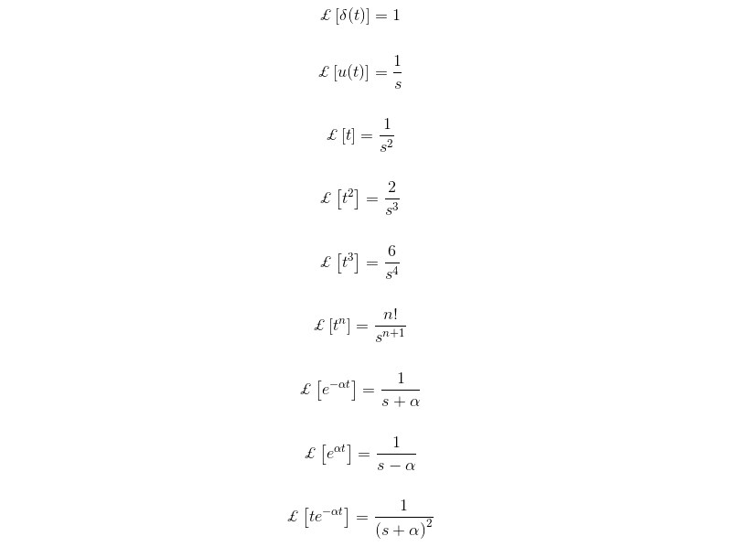
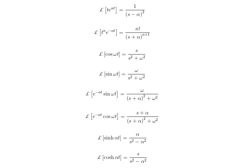
Transformation Calculator: Laplace Transform Table

A table containing information about Laplace transforms is always available to the engineer. Below is an example of such a table. From the following table, we will learn about the Laplace transform of various common functions.

Transformation Calculator: Method of Laplace Transform

An important part of control system engineering is the Laplace transformation. In order to study a control system, we need to perform the Laplace transform of the different functions (functions of time). Inverse Laplace is also important for determining a function’s Laplace form from its inverse. Inverse Laplace transforms and Laplace transforms are both useful for analyzing dynamic control systems. Linear systems benefit from Laplace transforms in several ways. Here are some of them:

Read Also: Quotient And Product Rule – Formula & Examples

Read Also: Difference Quotient – Formula, Calculator, Examples

Differentiation, integration, multiplication, frequency shifting, time scaling, time-shifting, convolution, conjugation, periodic function. Control systems are subject to two important theorems. They are:

1. Initial value theorem (IVT)
2. Final value theorem (FVT)

Laplace transforms a variety of functions, including impulse, unit impulse, step, unit step, shifted unit step, ramp, exponential decay, sine, cosine, hyperbolic sine, hyperbolic cosine, natural logarithm, and Bessel function. The greatest advantage of applying the Laplace transform is that it simplifies higher-order differential equations by converting them into algebraic equations.

There are certain steps that need to be followed in order to do a Laplace transform of a time function. In order to transform a given function of time \(f(t)\) into its corresponding Laplace transform, we have to follow the following steps:

• First multiply \(f(t)\) by \(e^{-st}\), \(s\) being a complex number \((s = \sigma + j\omega)\).
• Integrate this product w.r.t time with limits as zero and infinity. This integration results in the Laplace transformation of \(f(t)\), which is denoted by \(F(s)\).

Laplace transformation of $$f(t)=\mathscr{L}[f(t)]=F(s)=\int_{0}^{\infty}f(t)e^{-st}dt, when t \ge 0$$

The time function \(f(t)\) is obtained back from the Laplace transform by a process called inverse Laplace transformation and denoted by \(\mathscr{L}^{-1}\)

Inverse Laplace transformation of $$F(s)=\mathscr{L}^{-1}[F(s)]=\mathscr{L}^{-1}[\mathscr{L}f(s)]=f(s)$$

Transformation Calculator: Laplace Transform Properties

The main properties of Laplace Transform can be summarized as follows:

Linearity: Let \(C_1\), \(C_2\) be constants. \(f(t)\), \(g(t)\) be the functions of time, \(t\), then

$$\mathscr{L}\left\{C_1f(t)+C_2g(t) \right\}=\mathscr{L}\left\{C_1f(t) \right\}+\mathscr{L}\left\{C_2g(t) \right\}$$

Read Also: Derivative Of sin^2x, sin^2(2x) & More

Read Also: Horizontal Asymptotes – Definition, Rules & More

First shifting Theorem:

$$If\ \mathscr{L}\left\{f(t) \right\}=F(s)\ then\ \mathscr{L}\left\{e^{at}f(t) \right\}=F(s-a)$$

Change of scale property:

If\(\mathscr{L}\left\{f(t) \right\}=F(s),\ then\)

$$\mathscr{L}\left\{f(at) \right\}=\frac{1}{a}F(\frac{s}{a})$$

$$\mathscr{L}\left\{f(\frac{t}{a}) \right\}=aF(sa)$$

Differentiation:

If\(\mathscr{L}\left\{f(t) \right\}=F(s),\ then\)

$$\mathscr{L}\frac{d^n}{dt^n}\left\{f(t) \right\}=s^n\mathscr{L}\left\{f(t) \right\}-s^{n-1}f(0)-s^{n-2}f^1(0)-…f^{n-1}(0)$$

For example Let \(n=1\)

$$\mathscr{L}\frac{d^1}{dt^1}\left\{f(t) \right\}=s\mathscr{L}\left\{f(t) \right\}-f(0)$$

Integration:

If\(\mathscr{L}\left\{f(t) \right\}=F(s),\ then\)

$$\mathscr{L}\left[\int_{}^{}\int_{}^{}\int_{}^{}\int_{}^{}…\int_{}^{}f(t)dt^n \right]=\frac{1}{s^n}\mathscr{L}\left\{f(t) \right\}+\frac{}{}+\frac{f^{n-1}(0)}{s^n}+\frac{f^{n-2}(0)}{s^n}+…+\frac{f^{1}(0)}{s}$$

For example Let \(n=1\)

$$\mathscr{L}\left\{\int_{0}^{t}f(t)dt \right\}=\frac{1}{s}\mathscr{L}\left\{f(t) \right\}+\frac{f^{1}(0)}{s}$$

Time Shifting:

If \(\mathscr{L}\left\{f(t) \right\}=F(s)\), then the Laplace Transform of \(f(t)\) after the delay of time, \(T\) is equal to the product of Laplace Transform of \(f(t)\) and \(e^{-st}\) that is

$$\mathscr{L}\left\{f(t-T)u(t-T) \right\}=e^{-st}F(s)$$

Where \(u(t-T)\) denotes the unit step function.

Product:

If \(\mathscr{L}\left\{f(t) \right\}=F(s)\), then the product of two functions, \(f_1(t)\) and \(f_2(t)\) is

$$\mathscr{L}\left\{f_1(t)f_2(t) \right\}=\frac{1}{2\pi j}\int_{c-j\infty}^{c+j\infty}F_1(\omega)F_2(\omega)d\omega$$

Final Value Theorem:

If \(\mathscr{L}\left\{f(t) \right\}=F(s)\), then

$$\lim_{s \to \infty}f(t)=\lim_{s \to \infty}sF(s)$$

This theorem is applicable in the analysis and design of feedback control systems, as Laplace Transform gives a solution at initial conditions

Initial Value Theorem:

If \(\mathscr{L}\left\{f(t) \right\}=F(s)\), then

$$f(0^+)=\lim_{s \to \infty}sF(s)$$

Let us examine the Laplace transformation methods of a simple function \(f(t) = e^{\alpha t}\) for a better understanding of the matter.

Laplace transform of

$$e^{-\alpha t}=\mathscr{L}\left[e^{-\alpha t} \right]=\int_{0}^{\infty}e^{-\alpha t}.e^{-s t}dt=\int_{0}^{\infty}e^{-(s+\alpha)t}dt$$

$$\Rightarrow \mathscr{L}\left[e^{-\alpha t} \right]$$

$$=\frac{-1}{s+\alpha}\left[e^{-(s+\alpha)t} \right]_{0}^{\infty}$$

$$=\frac{-1}{s+\alpha}\left[e^{-(s+\alpha)\infty}-e^{-(s+\alpha)0} \right]$$

$$=\frac{-1}{s+\alpha}\left[0-1 \right]$$

$$=\frac{1}{s+\alpha}$$

Comparing the above solution, we can write,

Laplace transform of $$e^{\alpha t}=\mathscr{L}\left[e^{-(-\alpha t)} \right]=\frac{1}{s+(-\alpha)}=\frac{1}{s-\alpha}$$

Similarly, by putting \(\alpha = 0\), we get,

$$e^{0 t}=\mathscr{L}\left[e^0 \right]=\frac{1}{s+(0)}=\frac{1}{s}$$

Hence, Inverse laplace transform of \(\frac{1}{s}\)

$$\mathscr{L^{-1}}\left[\frac{1}{s} \right]=1$$

Similarly, by putting \(\alpha = j\omega\), we get,

Laplace transform of \(e^{j\omega t}\)

$$=\mathscr{L}\left[e^{j\omega t} \right]$$

$$=\frac{1}{s-j\omega}$$

Again \(e^{j\omega t}=\cos{\omega t}+j\sin{\omega t}\)

Therefore,

$$\mathscr{L}\left[e^{j\omega t} \right]=\mathscr{L}\left[\cos{\omega t}+j\sin{\omega t} \right]$$

$$=\mathscr{L}\left[\cos{\omega t} \right]+j\mathscr{L}\left[\sin{\omega t} \right]$$

Again,

$$\frac{1}{s-j\omega}=\frac{s+j\omega}{(s+j\omega)(s-j\omega)}$$

$$=\frac{s+j\omega}{(s^2-j^2\omega^2)}$$

$$=\frac{s+j\omega}{(s^2+\omega^2)}$$

$$=\frac{s}{(s^2+\omega^2)}+j\frac{\omega}{(s^2+\omega^2)}$$

Therefore, $$\mathscr{L}\left[\cos{\omega t} \right]=\frac{s}{(s^2+\omega^2)}\ and\ \mathscr{L}\left[\sin{\omega t} \right]=\frac{\omega}{(s^2+\omega^2)}$$

And thus,

$$\mathscr{L^{-1}}\left[\frac{s}{(s^2+\omega^2)} \right]=\cos{\omega t}\ and\ \mathscr{L^{-1}}\left[\frac{\omega}{(s^2+\omega^2)} \right]=\sin{\omega t}$$

Laplace Transform Examples

$$\pmb{\color{red}{Solve\ the\ equation\ using\ Laplace\ Transforms,}}$$

$$\pmb{\color{red}{f”(t)+3\ f'(t)+2\ f(t)=0,\ where\ f(0)=1\ and\ f'(0)=0}}$$

Using the table above, the equation can be converted into Laplace form:

$$\mathscr{L}\left[f”(t)+3\ f'(t)+2\ f(t) \right]=\mathscr{L}\left[f”(t) \right]+3\mathscr{L}\left[f'(t) \right]+2\mathscr{L}\left[f(t) \right]$$

Using the data that has been given in the question the Laplace form can be simplified.

$$(s^2 + 3s + 2)\mathscr{L}\left[f(t) \right]=s+3$$

Dividing by \((s^2 + 3s + 2)\) gives

$$\mathscr{L}\left[f(t) \right]=\frac{s+3}{s^2 + 3s + 2}$$

This can be solved using partial fractions, which is easier than solving it in its previous form. Firstly, the denominator needs to be factorized.

$$\frac{s+3}{s^2 + 3s + 2}=\frac{s+3}{(s+1)(s+2)}$$

$$\frac{s+3}{(s+1)(s+2)}=\frac{A}{(s+1)}+\frac{B}{(s+2)}$$

Cross-multiplying gives:

$$s+3=A(s+2)+B(s+1)$$

Next, the coefficients A and B need to be found \(s=-1,A=2,B=-1\)

Substituting in the equation:

$$\frac{2}{(s+1)}+\frac{-1}{(s+2)}$$

Where are Laplace Transforms used in Real Life?

Laplace’s Transform derives from Lerch’s Cancellation Law. In the Laplace Transform method, the function in the time domain is transformed into a Laplace function in the frequency domain. An algebraic equation can be used to solve this Laplace function. An Inverse Laplace Transform can be used to convert the solution back to the time domain.

As briefly mentioned above, this transform is most commonly used in control systems. In the study and analysis of systems like ventilation, heating, and air conditioning, the transforms are used. These systems are used in virtually every modern-day building.

Read Also: Domain And Range Calculator

For process control, Laplace transforms are also crucial. They help in analyzing variables that when changed produce the desired outcomes. Examples include experiments involving heat.

In addition to these two examples, Laplace transforms are used in a wide range of engineering applications and are extremely useful. They are useful in both electronic and mechanical engineering.

An electrical, mechanical, thermal, hydraulic, or another dynamic control system can be represented by a differential equation. According to the physical laws that govern a system, the differential equation for the system is derived. To facilitate the solution of a differential equation describing a control system, the equation is transformed into an algebraic form. A Laplace transformation is used to convert the time domain differential equation into a frequency domain algebraic equation.

Here is an analogy that may help in understanding Laplace. Imagine you come across a poem in English that you do not understand. You have a Spanish friend who is very good at understanding these poems. Therefore, you translate this poem into Spanish and send it to him, who then explains it in Spanish and sends it back to you. Having understood the Spanish explanation, you are able to transfer the meaning back to English and thus understand the English poem.

Disadvantages of the Laplace Transformation Method

The Laplace transform can only be applied to complex differential equations, and like all great methods, it has a disadvantage, which may not seem too significant. Therefore, this method can only be used to solve differential equations with known constants. You will need to come up with another method if you do not have any known constants in your equation.

History of Laplace Transforms

A transformation in mathematics involves the transformation of a function into another function that may not belong to the same domain. Those problems that cannot be directly solved can be solved with the transform method. The Laplace transform is named after the French mathematician and astronomer Pierre Simon Laplace.

In his contributions to probability theory, he used a similar transformation. After World War Two, it became very popular. Oliver Heaviside, an English electrical engineer, popularized this transform. In the 19th century, other famous scientists used it, such as Niels Abel, Mathias Lerch, and Thomas Bromwich.

More specifically, the history of the Laplace Transform can be traced back to 1744. During this time, another great mathematician named Leonhard Euler was investigating other types of integrals. He didn’t pursue it very far, however, and he left it behind. Among Euler’s admirers was Joseph Lagrange, who modified Euler’s work and completed further research.

The work of LaGrange caught Laplace’s attention 38 years later, in 1782 when Laplace picked up where Euler left off. In 1785, Laplace had a stroke of genius and changed the way we solve differential equations forever. Laplace worked on it, unlocking the true power of the Laplace transform until 1809 when he started using infinity as an integral condition.

Linear Transformation Calculator:

A linear transformation calculator is a tool used to perform calculations related to linear transformations in mathematics. Linear transformations involve the mapping of points or vectors from one coordinate system to another while preserving certain properties, such as straight lines and the origin.

Example:
Suppose you have a linear transformation defined as T(x, y) = (2x + y, 3x – y). By using the linear transformation calculator, you can input the coordinates (x, y) of a point and calculate the transformed coordinates (2x + y, 3x – y) based on the given linear transformation.

Laplace Transformation Calculator:

The Laplace transformation calculator is a tool used to compute the Laplace transform of a given function. The Laplace transform is a mathematical tool used to convert a function from the time domain to the frequency domain, which is useful in solving differential equations and analyzing systems.

Example:
Suppose you have a function f(t) = 3e^(2t) + sin(4t). By using the Laplace transformation calculator, you can input the function f(t) and calculate its Laplace transform F(s), which would be represented as F(s) = 3/(s – 2) + 4/(s^2 + 16).

Transformation Calculator Coordinates:

The transformation calculator coordinates is a tool used to perform calculations involving transformations of coordinates in geometry. It helps determine the new coordinates of a point after applying transformations such as translations, rotations, reflections, or dilations.

Example:
Suppose you have a point P(2, 3) and you want to translate it by (4, -1). Using the transformation calculator coordinates, you can input the initial coordinates (2, 3) and the translation vector (4, -1) to calculate the new coordinates after translation, which would be (6, 2).

Transformation Efficiency Calculator:

The transformation efficiency calculator is a tool used in molecular biology to determine the efficiency of a genetic transformation process. It calculates the percentage of successful transformation events or the number of transformed cells compared to the total number of cells subjected to the transformation.

Example:
In a genetic transformation experiment, you introduce a DNA construct into bacterial cells and want to determine the transformation efficiency. By using the transformation efficiency calculator, you input the number of transformed cells and the total number of cells, and it calculates the transformation efficiency as a percentage.

Transformation Calculator Matrix:

The transformation calculator matrix is a tool used to perform calculations involving matrix transformations. Matrix transformations are used in linear algebra to represent transformations of points or vectors using matrix multiplication.

Example:
Suppose you have a matrix transformation defined as T = [[2, 0], [0, 3]]. By using the transformation calculator matrix, you can input the coordinates of a point or a vector and calculate the transformed coordinates by multiplying the matrix T with the input vector.

Matrix Transformation Calculator:

The matrix transformation calculator is a tool used to perform calculations involving matrix transformations. It enables you to input a matrix representing a transformation and apply it to a given vector or set of vectors to obtain the transformed vectors.

Example:
Suppose you have a matrix transformation defined as T = [[1, 2], [3, 4]]. By using the matrix transformation calculator, you can input a vector, such as [2, 1], and calculate the transformed vector by multiplying it with the matrix T, resulting in [4, 9].

Transformation Calculator With Points:

The transformation calculator with points is a tool used to perform calculations involving transformations of points in geometry. It allows you to input the coordinates of a point and apply various transformations, such as translations, rotations, reflections, or dilations, to obtain the transformed coordinates.

Example:
Suppose you have a point P(3, -2) and you want to rotate it 90 degrees counterclockwise around the origin. By using the transformation calculator with points, you can input the initial coordinates (3, -2) and specify the rotation angle to calculate the new coordinates after the rotation, which would be (2, 3).

Transformation Of Functions Calculator:

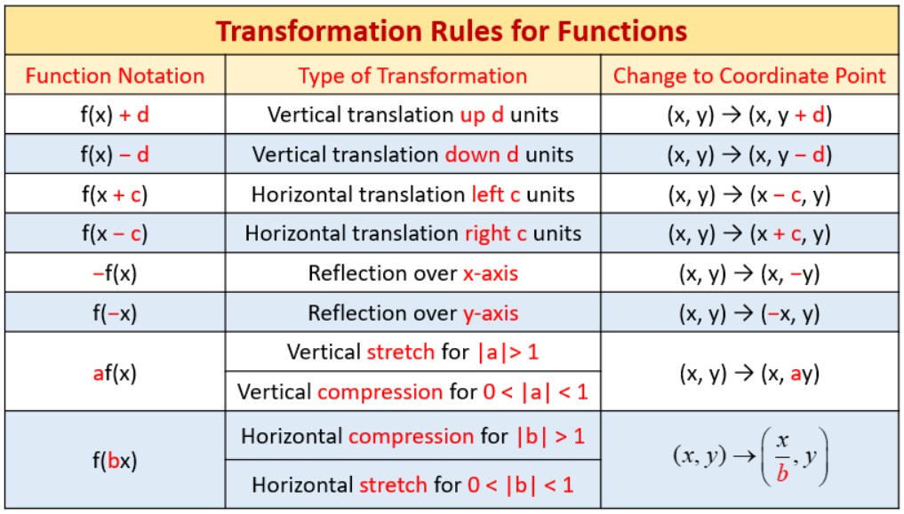
The transformation of functions calculator is a tool used to perform calculations involving transformations of mathematical functions. It helps determine the effect of transformations such as translations, stretches, compressions, or reflections on the graph of a given function.

Example:
Suppose you have the function f(x) = x^2 and you want to stretch it vertically by a factor of 3 and shift it 2 units to the left. Using the transformation of functions calculator, you can input the original function and specify the transformations to calculate the equation of the transformed function, which would be g(x) = 3(x + 2)^2.

Transformation Calculator Graph:

The transformation calculator graph is a tool used to visualize the graph of a function before and after applying transformations. It allows you to input a function and specify various transformations to observe the changes in the graph.

Example:
Suppose you have the function f(x) = sin(x) and you want to reflect it about the y-axis and stretch it vertically by a factor of 2. By using the transformation calculator graph, you can input the original function and specify the transformations to generate the graph of the transformed function, visualizing the reflection and vertical stretching.

FAQs

How do you find the transformation of a function?

The function transformation takes whatever is the basic function f (x) and then “transforms” it, which is simply a fancy way of saying that you change the formula a bit and move the graph around. This is three units higher than the basic quadratic, f (x) = x². That is, x² + 3 is f (x) + 3.

How do you find the transformation of a graph?

• Identify The Parent Function. Ernest Wolfe.
• Reflect Over X-Axis or Y-Axis.
• Shift (Translate) Vertically or Horizontally.
• Vertical and Horizontal Stretches/Compressions.
• Plug in a couple of your coordinates into the parent function to double-check your work.

What is the transformation of a graph?

The graph transformation process involves modifying an existing graph, or graphed equation, to produce variations of the original graph. Graphs can be translated, or moved about the xy plane; they can also be stretched, rotated, inverted, or any combination of these transformations.

How do you describe transformation?

A transformation is a way of changing the size or position of a shape. Every point in the shape is translated at the same distance in the same direction.

What is Transformation in quadratic equations?

Sometimes by looking at a quadratic function, you can see how it has been transformed from the simple function y=x². Then you can graph the equation by transforming the “parent graph” accordingly. For example, for a positive number c, the graph of y=x²+c is the same as graph y=x² shifted c units up.

What is a transformation in math example?

A transformation in math occurs when a shape, size, or position is altered. You can move pieces of a jigsaw puzzle by sliding them, flipping them, or turning them. Each of these moves changes the shape of the piece.

What Is The Energy Transformation Of A Solar Calculator?

A solar calculator utilizes solar panels to convert sunlight into electrical energy. The energy transformation in a solar calculator involves the conversion of solar energy (light energy) into electrical energy. The solar panels in the calculator absorb the sunlight and convert it into electrical energy, which is then used to power the calculator’s functions and display.

How To Do Z Transformation On The Calculator?

To perform a Z-transformation (also known as a standardization or normalization) on a calculator, you need to follow these steps:

1. Input the data set into your calculator.
2. Calculate the mean (average) of the data set.
3. Calculate the standard deviation of the data set.
4. Subtract the mean from each data point.
5. Divide the result of step 4 by the standard deviation.
6. The resulting values are the Z-scores, which represent the standardized values of the original data set.

By following these steps, you can perform the Z-transformation on a calculator and obtain the Z-scores for your data set.

What Kind Of Transformation Converts The Graph Of the Calculator?

The type of transformation that converts the graph of a function on a calculator depends on the specific transformation applied. Common types of transformations include translations, reflections, stretches or compressions, and combinations of these transformations.

For example:
– A translation shifts the graph horizontally or vertically.
– A reflection flips the graph over a line (e.g., x-axis or y-axis reflection).
– A stretch or compression alters the shape and size of the graph.
– A combination of these transformations may involve multiple changes to the graph.

The specific transformation applied will determine how the graph is converted or altered on the calculator.

What Energy Transformation Takes Place To Operate A Solar Powered Calculator?

In a solar-powered calculator, the energy transformation that takes place involves the conversion of solar energy into electrical energy. Solar energy from the sunlight is captured by solar panels, which contain photovoltaic cells. These cells use the photovoltaic effect to convert the sunlight into electrical energy. The electrical energy is then used to power the calculator’s functions and display, allowing it to operate without the need for traditional batteries.

How Do You Calculate Transformations?

To calculate transformations, you generally need the original object or function and the specific transformation applied. The steps to calculate transformations depend on the type of transformation being performed.

For geometric transformations, such as translations, rotations, reflections, or dilations:
1. Identify the original object’s coordinates or equation.
2. Apply the specific transformation rules (e.g., adding/subtracting values, multiplying/dividing by a factor, changing signs) to the original coordinates or equation.
3. Obtain the new coordinates or equation after the transformation.

For transformations of functions, such as translations, stretches, compressions, or reflections:
1. Start with the original equation of the function.
2. Apply the specific transformation rules to the equation (e.g., shifting horizontally/vertically, multiplying/dividing by a factor, changing signs).
3. Simplify the equation to obtain the transformed equation.

The calculations for transformations involve applying the appropriate rules or formulas based on the specific type of transformation being performed.

How Do You Find The Transformation Of A Graph?

To find the transformation of a graph, you need to compare the original graph to the transformed graph and identify the changes that have occurred. The specific steps may vary depending on the type of transformation involved.

For translations:
– Determine the horizontal and vertical shifts by comparing corresponding points on the original and transformed graphs.

For reflections:
– Identify the axis (x-axis, y-axis, or other) over which the reflection occurs.
– Observe how the points on the original graph relate to their reflections across the axis.

For stretches or compressions:
– Analyze the change in the shape and size of the graph by comparing the distances between corresponding points on the original and transformed graphs.

By visually examining the original and transformed graphs and analyzing the changes in their features, you can find and describe the transformation that has taken place.

What Are Transformation Rules?

Transformation rules are mathematical rules or formulas that describe how to perform specific transformations on objects or functions. These rules provide a systematic approach to apply changes such as translations, reflections, rotations, stretches, compressions, or combinations of these transformations.

For example:
– Translation: Add or subtract specific values to the coordinates of points or variables.
– Reflection: Change the sign of specific coordinates or variables based on the axis of reflection.
– Rotation: Apply formulas involving trigonometric functions to rotate points around a given angle or center.
– Stretch or Compression: Multiply or divide specific coordinates or variables by a factor to adjust the size or shape.

Transformation rules provide guidelines for performing transformations accurately and consistently, ensuring that the desired changes are applied correctly.