Table of Contents
Antiderivative Calculator is a free online tool that displays antiderivative (integration) functions. STUDYQUERIES’S online antiderivative calculator tool speeds up calculations, and it displays the integrated value in a fraction of a second.
How to Use the Antiderivative Calculator With Steps?
To use the antiderivative calculator, follow these steps:
- Step 1: Enter the function into the input field
- Step 2: Click the “Solve” button to get the antiderivative
- Step 3: In the new window, the antiderivative of the given function will be displayed
Antiderivative Calculator
What Is Antiderivative And Antiderivative Calculator?
The antiderivative is the name we sometimes, (rarely) give to the operation that goes backward from the derivative of a function to the function itself. Since the derivative does not determine the function completely (you can add any constant to your function and the derivative will be the same), you have to add additional information to go back to an explicit function as anti-derivative.

Thus we sometimes say that the antiderivative of a function is a function plus an arbitrary constant. Thus the antiderivative of \(cos(x)\) is \(sin(x)+c\).
The more common name for the antiderivative is the indefinite integral. This is the identical notion, merely a different name for it.
A wavy line is used as a symbol for it. Thus the sentence “the antiderivative of \(cos(x)\) is \(sin(x)+c\)” is usually stated as: the indefinite integral of \(cos(x)\) is \(sin(x)+c\), and this is generally written as
$$\int_{}^{}cos(x)dx=sin(x)+c$$
Read Also: Difference Quotient – Formula, Calculator, Examples
Read Also: Quotient And Product Rule – Formula & Examples
Actually, this is bad notation. The variable x that occurs on the right is a variable and represents the argument of the sine function. The symbols on the left merely say that the function whose antiderivative we are looking for is the cosine function. You will avoid confusion if you express this using an entirely different symbol (say y) on the left to denote this. The proper way to write this is then
$$\int_{}^{}cos(y)dy=sin(y)+c$$
What Is +C?
It is a reminder that the derivative of a constant is 0 so an anti-derivative as an inverse operation to a derivative is not completely determined. You can add any constant to an anti-derivative and get another one. Some believe that it was invented by pedants to torture students by penalizing them for occasionally ignoring this boring fact.
We can apply this to each term in a polynomial, and find its anti-derivative.
Thus, the anti-derivative of
$$3x^3-4x^2-x+7$$
is $$\frac{3x^4}{4} – \frac{4x^3}{3} – \frac{x^2}{2} + 7x + c$$
Students typically find this so easy that when they are forced to find such an anti-derivative on a test, often their minds are already focused on the next question, and they absent-mindedly forget and differentiate instead of anti-differentiating one or perhaps all terms. Please avoid this error.
Calculating Areas With Antiderivatives
A general method to find the area under a graph \(y=f(x)\) between \(x=a\)\ and \(x=b\)\ is given by the following important theorem.
Theorem
Let \(f(x)\) be a continuous real-valued function on the interval \([a,b]\). Then
$$\int_{a}^{b}f(x)dx=[F(x)]_b^a=F(b)−F(a)$$
where \(F(x)\) is any antiderivative of \(f(x)\).
The notation \([F(x)]_b^a\) is just a shorthand to substitute \(x=a\)\ and \(x=b\) into F(x) and subtract; it is synonymous with F(b)−F(a).
Read Also: Derivative Of sin^2x, sin^2(2x) & More
Read Also: Horizontal Asymptotes – Definition, Rules & More
Note that any antiderivative of \(f(x)\) will work in the above theorem. Indeed, if we have two different antiderivatives \(F(x)\)\ and \(G(x)\)\ of \(f(x)\), then they must differ by a constant, so \(G(x)=F(x)+c\) for some constant \(c\). Then we have to get the same answer whether we use \(F\)\ or \(G\), since
\(G(b)−G(a)=(F(b)+c)−(F(a)+c)=F(b)−F(a)\).
We give a proof of the theorem, assuming our previous statements:
- The derivative of the area function is \(f(x)\(
- Any two antiderivatives of \(f(x)\( differ by a constant.
\(\color{red}{Find \int_{0}^{5}(x^2+1)dx.}\)
\(\int_{0}^{5}(x^2+1)dx\)
\(=[\frac{1}{3}(x^3)+x]_0^5\)
\(=[\frac{1}{3}(5^3)+5]-[\frac{1}{3}(0^3)+0]\)
\(=\frac{125}{3}+5\)
\(=\frac{140}{3}\)
How Can We Calculate Velocity And Acceleration With Antiderivative?
For now, let’s look at the terminology and notation for antiderivatives, and determine the antiderivatives for several types of functions. We examine various techniques for finding antiderivatives of more complicated functions later in the text (Introduction to Techniques of Integration).
This section assumes you have enough background in calculus to be familiar with integration. In Instantaneous Velocity and Speed and Average and Instantaneous Acceleration, we introduced the kinematic functions of velocity and acceleration using the derivative.
By taking the derivative of the position function we found the velocity function, and likewise, by taking the derivative of the velocity function we found the acceleration function. Using integral calculus, we can work backward and calculate the velocity function from the acceleration function, and the position function from the velocity function.
Kinematic Equations from Integral Calculus
Let’s begin with a particle with an acceleration \(a(t)\) is a known function of time. Since the time derivative of the velocity function is acceleration,
$$\frac{d}{dt}v(t)=a(t)$$,
we can take the indefinite integral of both sides, finding
$$\int_{}^{}\frac{d}{dt}v(t)dt=\int_{}^{}a(t)dt+C_1$$
where \(C_1\) is a constant of integration. Since \(\int_{}^{}\frac{d}{dt}v(t)dt=v(t)\), the velocity is given by
$$v(t)=\int_{}^{}a(t)dt+C_1$$
Similarly, the time derivative of the position function is the velocity function,
$$\frac{d}{dt}x(t)=v(t)$$
Thus, we can use the same mathematical manipulations we just used and find
$$x(t)=\int_{}^{}v(t)dt+C_2$$
where \(C_2\) is the second constant of integration.
We can derive the kinematic equations for a constant acceleration using these integrals. With \(a(t) = a\)\ constant, and doing the integration in, we find
$$v(t)=\int_{}^{}a(t)dt+C_1=at+C_1$$
If the initial velocity is \(v(0) = v_0\), then
\(v_0=0+C_1\)
Then, \(C_1 = v_0\) and
\(v(t)=v_0+at\),
which is (Equation). Substituting this expression gives
\(x(t)=\int_{}^{}(v_0+at)dt+C_2\)
Doing the integration, we find
\(x(t)=v_0t+\frac{1}{2}at^2+C_2\)
If \(x(0) = x_0), we have
\(x_0=0+0+C_2\);
so, \(C_2 = x_0\). Substituting back into the equation for \(x(t)\), we finally have
\(x(t)=x_0+v_0t+\frac{1}{2}at^2\).
Read Also: Domain And Range Calculator
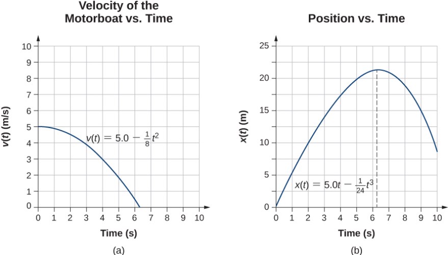
\(\color{red}{A\ motorboat\ is\ traveling\ at\ a\ constant\ velocity\ of\ 5.0 \frac{m}{s}}\),
\(\color{red}{when\ it\ starts\ to\ decelerate\ to\ arrive\ at\ the\ dock.\ Its\ acceleration\ is\ a(t)=−\frac{1}{4}t(\frac{m}{s^2})}\).
- What is the velocity function of the motorboat?
- At what time does the velocity reach zero?
- What is the position function of the motorboat?
- What is the displacement of the motorboat from the time it begins to decelerate to when the velocity is zero?
- Graph the velocity and position functions.
Strategy
- To get the velocity function we must integrate and use initial conditions to find the constant of integration.
- We set the velocity function equal to zero and solve for t.
- Similarly, we must integrate to find the position function and use initial conditions to find the constant of integration.
- Since the initial position is taken to be zero, we only have to evaluate the position function at \(t=0\).
We take \(t = 0\) to be the time when the boat starts to decelerate.
1: From the functional form of the acceleration we can solve to get \(v(t)\):
$$v(t)=\int_{}^{}a(t)dt+C_1$$
$$=\int_{}^{}(−\frac{1}{4}t)dt+C_1$$
$$=−\frac{1}{8}t^2+C_1$$
At \(t = 0\) we have \(v(0) = 5.0 \frac{m}{s} = 0 + C_1, so C_1 = 5.0 \frac{m}{s}\) or
$$v(t)=5.0\frac{m}{s}−\frac{1}{8}t^2$$
2: $$v(t)=0$$
$$0=5.0\frac{m}{s}−\frac{1}{8}t^2\Longrightarrow t=6.3s$$
3: $$x(t)=\int_{}^{}v(t)dt+C_2$$
$$=\int_{}^{}(5.0−\frac{1}{8}t^2)dt+C_2$$
$$=5.0t−\frac{1}{24}t^3+C_2$$
At \(t = 0\), we set \(x(0) = 0 = x_0\), since we are only interested in the displacement from when the boat starts to decelerate. We have
\(x(0)=0=C_2\). Therefore, the equation for the position is
$$x(t)=5.0t−\frac{1}{24}t^3$$
4: Graph A is a plot of velocity in meters per second as a function of time in seconds. Velocity is five meters per second in the beginning and decreases to zero. Graph B is a plot of position in meters as a function of time in seconds. The position is zero at the beginning, increases reaching a maximum between six and seven seconds, and then starts to decrease.
Initial Value Problems
We look at techniques for integrating a large variety of functions involving products, quotients, and compositions later in the text. Here we turn to one common use for antiderivatives that arises often in many applications: solving differential equations.
A differential equation is an equation that relates an unknown function and one or more of its derivatives. The equation
$$\frac{dy}{dx}=f(x)$$
is a simple example of a differential equation. Solving this equation means finding a function y with a derivative \(f\). Therefore, the solutions of Equation are the antiderivatives of \(f\). If \(F\) is one antiderivative of \(f \), every function of the form \(y=F(x)+C\) is a solution of that differential equation. For example, the solutions of
$$\frac{dy}{dx}=6x^2$$
are given by
$$y=\int_{}^{}6x^2dx=2x^3+C$$
Sometimes we are interested in determining whether a particular solution curve passes through a certain point \((x_0,y_0)\) —that is, \(y(x_0)=y_0\). The problem of finding a function y that satisfies a differential equation
$$\frac{dy}{dx}=f(x)$$
with the additional condition \(y(x_0)=y_0\) is an example of an initial-value problem. The condition \(y(x_0)=y_0\) is known as an initial condition. For example, looking for a function \(y\) that satisfies the differential equation
$$\frac{dy}{dx}=6x^2$$
and the initial condition \(y(1)=5\) is an example of an initial-value problem. Since the solutions of the differential equation are \(y=2x^3+C\), to find a function y that also satisfies the initial condition, we need to find \(C\) such that \(y(1)=2(1)^3+C=5\). From this equation, we see that \(C=3\), and we conclude that \(y=2x^3+3\) is the solution of this initial-value problem as shown in the following graph.
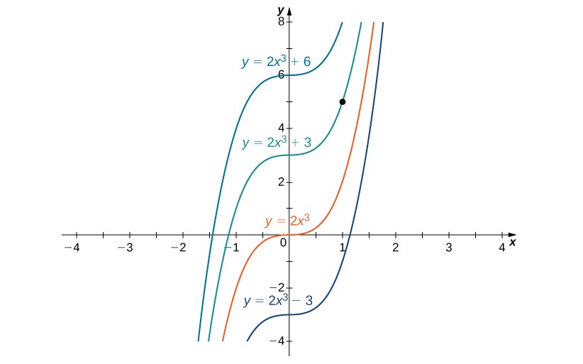
Some of the solution curves of the differential equation \(\frac{dy}{dx}=6x^2\) are displayed. The function \(y=2x^3+3\) satisfies the differential equation and the initial condition \(y(1)=5\).
Antiderivative Calculator With Steps:
An antiderivative calculator with steps is a tool that helps find the antiderivative (also known as the indefinite integral) of a given function. It not only provides the numerical value of the antiderivative but also shows the step-by-step process of how the antiderivative is computed. This allows users to understand and learn the technique of finding antiderivatives.
Example:
Suppose you want to find the antiderivative of the function f(x) = 2x^3 + 5x^2 – 3x. Using the antiderivative calculator with steps, it will show the step-by-step process, such as applying the power rule and the constant rule, resulting in the antiderivative F(x) = (1/2)x^4 + (5/3)x^3 – (3/2)x^2 + C, where C is the constant of integration.
General Antiderivative Calculator:
A general antiderivative calculator is a tool that calculates the antiderivative of a function using general antiderivative formulas and rules. It provides the result without specifying the constant of integration. Instead, it includes the “+ C” term to represent the constant of integration that can take any value.
Example:
If you input the function f(x) = 3x^2 + 2x into a general antiderivative calculator, it will give you the result F(x) = x^3 + x^2 + C, where C represents the constant of integration.
Second Antiderivative Calculator:
A second antiderivative calculator is a tool that calculates the antiderivative of a function twice, resulting in a second antiderivative. This is achieved by applying the antiderivative operation twice to the given function.
Example:
Let’s say you have the function f(x) = 6x^3 + 2x^2 + 5x. By using a second antiderivative calculator, you would apply the antiderivative operation twice, resulting in the second antiderivative G(x) = (1/4)x^4 + (2/3)x^3 + (5/2)x^2 + Cx + D, where C and D are constants of integration.
Find Antiderivative Calculator:
A find antiderivative calculator is a tool that determines the antiderivative of a given function. It evaluates the function and provides the corresponding antiderivative without showing the step-by-step process.
Example:
Suppose you want to find the antiderivative of the function f(x) = 4x^2 – 3x + 2. Using a find antiderivative calculator, it will directly give you the result F(x) = (4/3)x^3 – (3/2)x^2 + 2x + C, where C is the constant of integration.
Reverse A Derivative Calculator:
A reverse derivative calculator, also known as an antiderivative calculator, is a tool that finds the antiderivative of a given derivative. It works in the opposite direction of a standard derivative calculator, allowing you to recover the original function.
Example:
If you have the derivative f'(x) = 3x^2 – 2x + 1, you can use a reverse derivative or antiderivative calculator to find the original function f(x) by finding its antiderivative. The result will be f(x) = x^3 – x^2 + x + C, where C is the constant of integration.
Antiderivative Of -cos(x):
The antiderivative of -cos(x) is calculated by finding the function whose derivative is equal to -cos(x). In this case, the ant
iderivative of -cos(x) is sin(x) + C, where C is the constant of integration.
Most General Antiderivative Calculator:
A most general antiderivative calculator is a tool that calculates the antiderivative of a function by including all possible constant values in the result. It represents the entire family of antiderivatives by including an arbitrary constant, allowing users to explore the range of possible solutions.
Example:
If you input the function f(x) = 2x into a most general antiderivative calculator, it will give you the result F(x) = x^2 + C, where C represents any constant value.
Antiderivative Of 1:
The antiderivative of 1, denoted as ∫1 dx, is x + C, where C is the constant of integration. This is because the derivative of x + C is equal to 1.
Note: In all the examples above, “C” represents the constant of integration, which is added when finding antiderivatives since the derivative of a constant is zero. The constant allows for the inclusion of all possible solutions when integrating.
FAQs
What is an antiderivative calculator?
Anti-derivative Calculator is an online tool used to calculate the value of a given indefinite integral. Integration can be used to find the area under a curve. It can also be used to determine the volume of a three-dimensional solid shape.
Is integral the same as antiderivative?
Antiderivatives are related to definite integrals through the fundamental theorem of calculus: the definite integral of a function over an interval is equal to the difference between the values of an antiderivative evaluated at the endpoints of the interval.
What are Antiderivatives used for?
An antiderivative is a function that reverses what the derivative does. One function has many antiderivatives, but they all take the form of a function plus an arbitrary constant. Antiderivatives are a key part of indefinite integrals.
What is a general antiderivative?
General Antiderivative The function F(x) + C is the General Antiderivative of the function f(x) on an interval I if F (x) = f(x) for all x in I and C is an arbitrary constant. Indefinite Integral The Indefinite Integral of f(x) is the General Antiderivative of f(x).
What is antiderivative sin?
The general antiderivative of sin(x) is −cos(x)+C . With an integral sign, this is written: ∫sin(x) dx=−cos(x)+C .
How To Find Antiderivative On Calculator?
To find an antiderivative on a calculator, you can use the built-in functions or features designed for integration. Here are the general steps:
1. Enter the function for which you want to find the antiderivative into the calculator.
2. Look for a specific key or menu option on the calculator that is related to integration or antiderivatives.
3. Use the appropriate function or command to calculate the antiderivative of the given function.
4. The calculator will display the result, typically in the form of a new function with the “+ C” term representing the constant of integration.
The specific procedure may vary depending on the calculator model and brand, so consult the user manual or instructions for your specific calculator to find the integration function.
How To Take An Antiderivative On A Calculator?
To take an antiderivative on a calculator, you need to follow these steps:
1. Enter the function you want to integrate into the calculator.
2. Locate the appropriate integration or antiderivative function on the calculator.
3. Use the function or command to calculate the antiderivative.
4. The calculator will provide the result, typically in the form of a new function with the “+ C” term representing the constant of integration.
Make sure to use the correct syntax and follow the instructions provided by the calculator’s manual or guide.
How To Find An Antiderivative Function In A Calculator?
To find an antiderivative function in a calculator, you need to follow the specific procedures outlined by the calculator’s manufacturer. Most scientific or graphing calculators have built-in functions for finding antiderivatives or performing integration.
Refer to the user manual or guide that accompanies your calculator to locate the integration or antiderivative function and understand how to input the function you want to integrate. By following the instructions, you can find the antiderivative function using the calculator.
What Is The Antiderivative Of 1-1/2X Calculator?
The antiderivative of 1 – (1/2)x is calculated as follows:
∫(1 – (1/2)x) dx = x – (1/4)x^2 + C
The result is a new function that represents the antiderivative, where C represents the constant of integration.
How To Find Antiderivative?
To find an antiderivative manually (without a calculator), you can use various integration techniques and rules. Here are the general steps:
1. Identify the function for which you want to find the antiderivative.
2. Apply the power rule, product rule, chain rule, or other integration techniques based on the function’s structure.
3. Integrate each term or part of the function separately, treating constants as factors.
4. Add the “+ C” term to the end of the integrated function to represent the constant of integration.
The process of finding antiderivatives can involve more advanced integration techniques, such as substitution or integration by parts, depending on the complexity of the function.
How To Put Antiderivative In Calculator?
To put an antiderivative in a calculator, you usually input the original function, and the calculator will calculate the antiderivative for you. The exact steps may vary depending on the calculator model, but in general:
1. Enter the original function into the calculator.
2. Use the appropriate integration or antiderivative function or command on the calculator.
3. The calculator will compute the antiderivative and display the result, typically in the form of a new function with the “+ C” term representing the constant of integration.
Ensure that you understand the syntax and functions specific to your calculator by referring to the user manual or guide provided with the calculator.